Basic SkyProj Interface

Getting Started

SkyProj is an interface linking matplotlib with PROJ to create good looking and interactive visualizations of astronomical map data, in particular HealSparse and HEALPix maps. It has its origins in cartosky, which was built on cartopy and some of the features may be familiar to users of cartopy. However, it has diverged significantly as the needs of mapping the sky are somewhat different from mapping the Earth.

The fundamental base class for SkyProj is the skyproj.Skyproj() sky projection. This class is a container for a matplotlib axis (for plotting); a matplotlib axis artist (for drawing gridlines and labels); a coordinate reference system (CRS) which describes a particular map projection; and a large number of methods for plotting maps, lines, polygons, and colorbars. The Skyproj() class is designed to create projections that are accurate and attractive for full-sky and zoomed maps.

Creating a Default Skyproj()

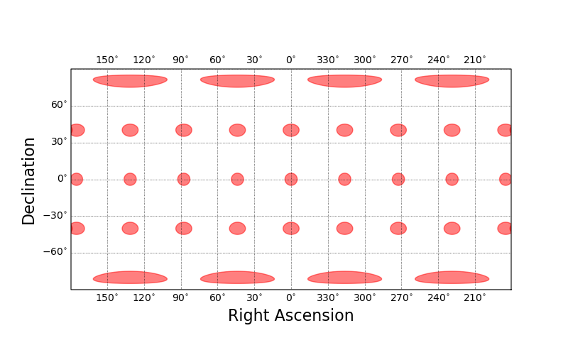
The default projection for a skyproj.Skyproj() is the Plate carrée (literally “flat square”) or equirectangular projection. This projection maps longitude (right ascension) and latitude (declination) directly onto a grid. It is neither conformal (angle preserving) or equal area, so is not particularly recommended for plotting astronomical data.

import matplotlib.pyplot as plt
import skyproj

# Create a figure and an associated axis.
fig, ax = plt.subplots(figsize=(8, 5))
# We can specify the axis in the instantiation of Skyproj(), or can
# let it use the "current axis".
sp = skyproj.Skyproj(ax=ax)
# Draw Tissot's Indicatrices to show the distortion of the projection.
sp.tissot_indicatrices()
plt.show()

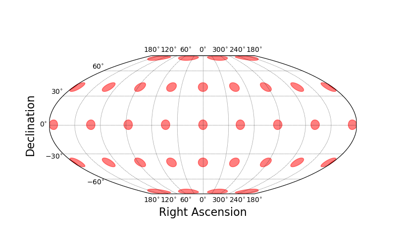
Creating an Equal-Area McBrydeSkyproj()

The McBryde-Thomas Flat Polar Quartic projection is an equal-area pseudocylindrical projection that has been used for the Dark Energy Survey.

The McBryde projection can be accessed with skyproj.McBrydeSkyproj() class.

import matplotlib.pyplot as plt
import skyproj

fig, ax = plt.subplots(figsize=(8, 5))
sp = skyproj.McBrydeSkyproj(ax=ax)
sp.tissot_indicatrices()
plt.show()

For further information on other projections available, see SkyProj Projections.

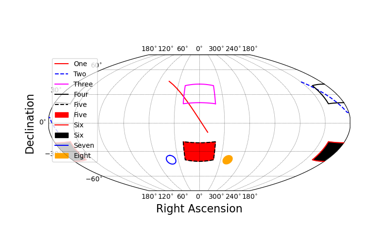
Drawing Lines and Polygons

It is easy to draw lines, polygons, and circles on a Skyproj() object. When specifying connected points or polygon edges, they will be connected with a geodesic interpolation. Similarly, circles are drawn as a connected locus of points that are all equidistant from the center as computed from geodesics.

import matplotlib.pyplot as plt
import skyproj

fig, ax = plt.subplots(figsize=(8, 5))
sp = skyproj.McBrydeSkyproj(ax=ax)

# Draw two geodesics, one of which will wrap around.
sp.plot([-10., 45.], [-10., 45.], 'r-', label='One')
sp.plot([170., 210.], [-10., 45.], 'b--', label='Two')

# Draw two unfilled polygons, one of which will wrap around.
sp.draw_polygon([-20, 20, 20, -20], [20, 20, 40, 40],
                edgecolor='magenta', label='Three')
sp.draw_polygon([160, 200, 200, 160], [20, 20, 40, 40],
                edgecolor='black', label='Four')

# Draw two filled polygons, one of which will wrap around.
sp.draw_polygon([-20, 20, 20, -20], [-20, -20, -40, -40],
                edgecolor='black', facecolor='red', linestyle='--', label='Five')
sp.draw_polygon([160, 200, 200, 160], [-20, -20, -40, -40],
                edgecolor='red', facecolor='black', linestyle='-', label='Six')

# Draw a circle
sp.circle(40.0, -40.0, 5.0, label='Seven')
sp.circle(-40.0, -40.0, 5.0, color='orange', label='Eight', fill=True)

# Draw one open ellipse and one rotated, filled ellipse.
# ellipse expects (ra, dec, r_A, r_B, theta)  [degrees]
# where r_A=Semi-major axis, r_B=semi-minor axis, theta=position angle.
sp.ellipse(60, 15, 10, 4, 0, color='green', label='Nine')
sp.ellipse(300, 15, 15, 2, 45, fill=True, color='red', label='Ten')

# Make a legend
sp.legend()
plt.show()

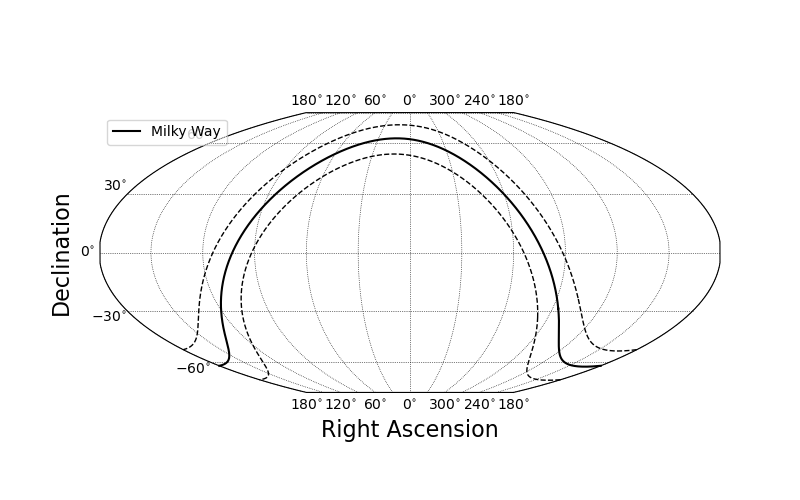
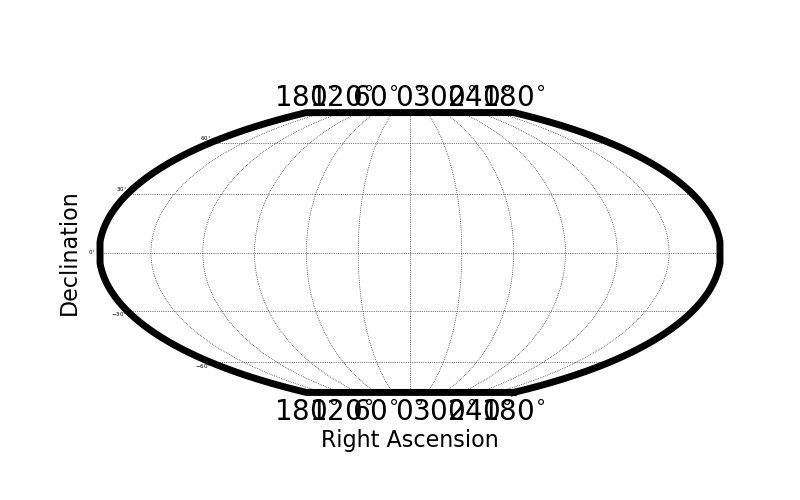
Drawing the Milky Way

Included in SkyProj is a convenient way of representing the Milky Way Galaxy. The default is to plot a thick line along the Galactic equator, and two dashed lines at +/- 10 degrees.

import matplotlib.pyplot as plt
import skyproj

fig, ax = plt.subplots(figsize=(8, 5))
sp = skyproj.McBrydeSkyproj(ax=ax)
sp.draw_milky_way(label='Milky Way')
sp.legend()
plt.show()

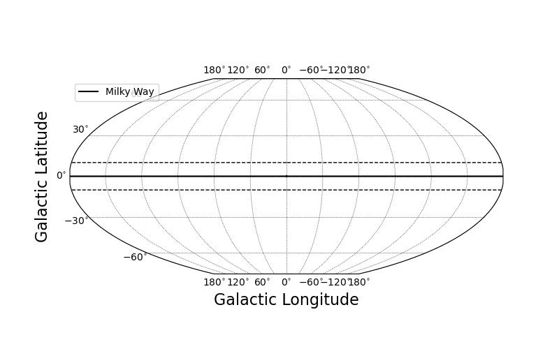
It is also possible to specify that the default plotting units should be Galactic coordinates rather than Equatorial coordinates. When using draw_milky_way(), it will plot in Galactic coordinates.

import matplotlib.pyplot as plt
import skyproj

fig, ax = plt.subplots(figsize=(8, 5))
sp = skyproj.McBrydeSkyproj(ax=ax, galactic=True, longitude_ticks='symmetric')
sp.draw_milky_way(label='Milky Way')
sp.legend()
plt.show()

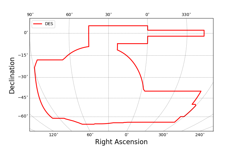
Survey Maps

SkyProj includes convenient survey classes which have the ability to plot survey outlines. In addition, these survey classes have convenient preset projections and extents set that are appropriate for plotting the survey. See SkyProj Surveys for further information on what surveys are available (and feel free to file an issue or make a PR for your favorite survey).

import matplotlib.pyplot as plt
import skyproj

fig, ax = plt.subplots(figsize=(8, 5))
sp = skyproj.DESSkyproj(ax=ax)
sp.draw_des(label='DES')
sp.legend()
plt.show()

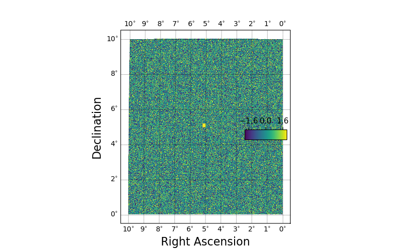
Plotting HealSparse and HEALPix Maps

Plotting HealSparse maps can be performed with the draw_hspmap() method on a Skyproj() subclass. The default setting for drawing a map is to automatically zoom in on the ra/dec range of the map to be plotted. For speed and efficiency, map plotting in SkyProj is performed by first rasterizing the input map at a resolution appropriate for the given plot. For more details on plotting HealSparse and HEALPix maps, see SkyProj HealSparse and Healpix Mapping.

import matplotlib.pyplot as plt
import numpy as np
import healsparse as hsp
import skyproj

# Make a square noise field.
hspmap = hsp.HealSparseMap.make_empty(32, 4096, np.float32)
poly = hsp.geom.Polygon(ra=[0.0, 10.0, 10.0, 0.0], dec=[0.0, 0.0, 10.0, 10.0], value=1.0)
pixels = poly.get_pixels(nside=hspmap.nside_sparse)
hspmap[pixels] = np.random.normal(size=pixels.size).astype(np.float32)
# Add in a central square of fixed value.
poly2 = hsp.geom.Polygon(ra=[5, 5.2, 5.2, 5.0], dec=[5, 5.0, 5.2, 5.2], value=3.0)
pixels2 = poly2.get_pixels(nside=hspmap.nside_sparse)
hspmap[pixels2] = 3.0

fig, ax = plt.subplots(figsize=(8, 5))
sp = skyproj.McBrydeSkyproj(ax=ax)
im, lon_raster, lat_raster, values_raster = sp.draw_hspmap(hspmap)
sp.draw_inset_colorbar()
plt.show()

Interactivity

All maps created by SkyProj are interactive using the standard matplotlib interactivity tools. Zooming and panning are supported through the standard widgets. When the map is zoomed, any healsparse or HEALPix map will be re-rasterized at the new resolution. In this way, one can view a high resolution map over the full sky without rendering every tiny pixel; when zoomed, more detail will appear.

The default behavior on zoom is for the colorbar to be rescaled based on the range of map pixels shown in the current frame. This functionality can be turned off by either instantiating the SkyProj() subclass with autrescale=False or by using sp.set_autorescale(False).

In addition, the default behavior on zoom is for the map to retain the original projection. When zooming in to a small region far from the central longitude this can lead to large distortion (as seen in the Tissot Indicatrices of the McBryde projection above). There is currently experimental support for reprojecting on the current displayed central longitude by hitting R (for Reproject) when the mouse is within the plot window. Performing the reprojection may be slow, and there are some cases where it can go awry. When the zoom is below 1 degree across the reprojection will use a Gnomonic (tangent-plane) projection which has sufficiently small distortion at all locations.

Plotting Customization

Much of the plotting functionality is decided by SkyProj itself. However, there is a lot of customization available. The fonts, font sizes, tick label sizes, etc, are all determined by the matplotlib RC parameter dictionary. A few of these in particular should be highlighted:

• xticks.labelsize: Sets the label size for the x (longitude) ticks on the plot.

• yticks.labelsize: Sets the label size for the y (latitude) ticks on the plot.

• axes.linewidth: Sets the width of the boundary of the full plot.

• axes.labelsize: Sets the size of the x/y (lon/lat) labels; this will default to 16 unless specifically overridden with an rcparams.

These values (and any others) can be overridden at the time of map instantiation with a temporary dictionary, like so:

import matplotlib.pyplot as plt
import skyproj

# These values are comically exaggerated for effect.
rcparams = {'xtick.labelsize': 20,
            'ytick.labelsize': 4,
            'axes.linewidth': 5}

fig, ax = plt.subplots(figsize=(8, 5))
sp = skyproj.McBrydeSkyproj(ax=ax, rcparams=rcparams)
plt.show()

There are additional SkyProj specific customization options that are not controlled via the matplotlib RC parameter dictionary. These include the number of grid lines in the longitude and latitude direction, as well as minimum spacing between latitude tick labels to help prevent label clashes. These options are controlled at initialization time via keyword parameters, and include:

• longitude_ticks: Label longitude ticks from 0 to 360 degrees (positive) or from -180 to 180 degrees (symmetric).

• n_grid_lon: The number of grid lines to use in the longitude direction (x in rectangular-style projections). The default is the axis ratio of the plot multiplied by the number of latitude grid lines.

• n_grid_lat: The number of grid lines to use in the latitude direction (y in rectangular-style projections). The default is 6 lines.

• min_lon_ticklabel_delta: The minimum relative spacing between longitude tick labels (relative to the width of the axis). Smaller values yield closer tick labels (and the potential for clashes), and larger valus yield more spacing between tick labels.